GIS Lab 10 - 16c

The only difference of this layout was to change the number from 2707 to 4001. Also about the chart as I tried to another and field calculate for the Acres but for some minor reason it didn't want to calculate the numbers into the attribute chart.

GIS Lab 10 -16a

Chapter 16a is the tutorial of editing features and attributes, also it shows features like deleting and modifying the parcel areas within the edit session.

GIS Lab 10 - 16b

16b splitting and modifying features here it depicts that 2707 has split in to two areas of parcels. With the shape being the same 2707 polygon, the Shape area 2707 Big -94611.381 and 2707 Small -12637.322 .

In this exercise, the task is to remove the duplex from the cul-de-sac. Due to the reason that an owner bought the other half and now wants to join both parcel areas into one structure. As the process goes by we end up with Shape area of 17354.414 of parcel area 2855.

GIS Lab 10 - 15b

15b Editing Parcels while using the feature construction tools to digitize features representing the lands parcels that consist in this exercise.

This parcel is drawn from my specifications while following the tutorials of this exercise. Now you notice that I added and proposed 2 parcels to the subdivision for the City data geodatabase.

GIS Lab 10 - 15a

15a consists of creating and editing data such as digitizing water lines to connect undeground valves. In this subdivision thats under construction layers of water valves, fire hydrants, water lines and parcels are common usage for this exercise. Using the cursor valve lines from 813 to 763 to 831 and ending it up to the hydrant.

GIS Lab 10 - Tool Map

The point data set from chapter 9a, the Louisiana parishes while on the spatial statistics tool I decided to choose the Average Nearest Neighbor index from the Analyzing Patterns tool set. Its purpose is based on the average distance from each feature to its nearest neighboring feature. 

 

 

- Nearest Neighbor Ratio: 0.325 P-Value: 0.000 Z-Score: -31.770

GIS Lab 9 - 12c

Lastly, calculatiing attribute values for all records for Lease F for the bidding came out like 1,052.08379, so the harvest is just over a billion (statistics). 

GIS Lab 9 - 12b

Overlaying Data where the harvestable area of lease F is composed of all polygons in the Final layer that have a value of -1 in the no cut area set.

GIS Lab 9 - 12a

Using Buffering to determine the value of harvestable land in Lease F (above). The Buffer layers define the areas within which trees cannot be cut.

GIS Lab 9 - 11d

Exporting Data, so nests are contained within polygons, so instead of clipping or dissolving, we will export the selected sets to make the Goshawk Nests layer to the point Data.

GIS Lab 9 - 11c

Clipping layers in five lease areas that contains a segment of 1,556 streams. Clipped on the left side and right the segment streams ready to be clip.

 

From 1,566 to 358 streams clipped upon this lease stand while using the StreamsF layer. 

GIS Lab 9 - 11b

Adding graphs to the layout page to represent the Values of the forest stand into the lease areas.

GIS Lab 9 - 11a

The Lease areas of the five stands from the Forest Service, in dissolving mode/image. 

The Forest Service in present of five adjacent areas that are also lease areas.

GIS Lab 8 Map 9b

Joining and Relating tables part 2. This time in the state of Louisiana, we will go to the Lower Mississippi Buffer to see the section of Pits_75 but relating tables. Once after relating tables with the Pits and Metals to the Remedial Actions and IDNumbers. Witness, you can see the record points of 3 pits that contain lead.

GIS Lab 8 Map 9a

Joining and Relating tables, a map of Louisiana showing parishes, navigable, waterways, and pits. But now with joining the tables of Remedial-Actions to thier IDNumbers it will show that Pits need to be repaired or removed that are moslty located in  parishes of the southeastern tip of the state. 

GIS Lab 7 Map

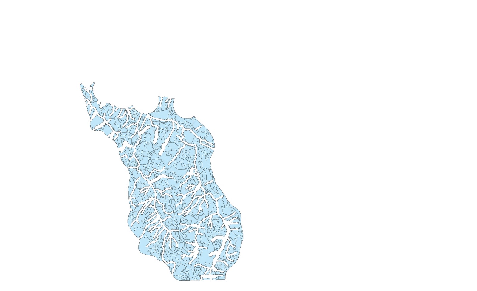
The Data Mining project was kind of difficult at first especially looking for the right data that needs to be downloaded. Here depicts like 3 types of  spatial datasets that is used. For instance, DEM Data, Hydrography Data, Census Data and a Wetlands Data. All of them used the projection of North America 1983 11N to be visible and match with the corresponding datasets that are put together.  

GIS Lab 6 - 19d Map

Lastly adding the final thouches, once everything inserted and complete within the map, I add a picture of a Tiger from the Insert menu.

GIS Lab 6 - 19c Map

The depiction of this map is to review the proposal and the map needs to familiar with the geography of India. So that's why I inserted legends, scale bars, and north arrows because they are necessary for interpreting a map for geographic orentation.

GIS Lab 6 - 19b Map

Here we see a title that portrays the meaning of what the project is about. Before moving on the data frame on the right depicts the use of vegetation and forest for residential and commercial use. The frame on the left depicts Proposed reserves where high priorities are in red and low priorities are in blue.

GIS Lab 6 - 19a Map

First of all, this project consists of tiger conservation and existing reserves along vegetation corridors. I began to work with three Data Frames that were given to me but needed to be aligned. The bottom data frame is the Overview frame, the data frame on the left is the Existing reserves frame (Bio), and the one on the right will be the Proposed reserves frame (Tiger).

GIS Lab 6 - 18a Map 2

This map represents the Continent of Asia, its suppose to be before the map of Asia where is depicts the country of the Philippines. Then it will follow through to understand where the Philippines location is.

GIS Lab 6 - 18c Map

Once called the map of Asia, now is known as the Path of Typhoon Etang map. Notice on the last map, the typhoon passes closely to the Philippines, but on this map it now has direction, date, and time. Heading northeast of the last position of the typhoon, it depicts the time and speed of its last recorded position. 

GIS Lab 6 - 18b Map

The map represents the in  showing the location, speed, and path of Typhoon Etang (dark blue). With the latitude and longitude coordinates, it shows where the typhoon has been at different times.

GIS Lab 6 - 18a Map

The Philippines, had to change the graticule and interval values to from 10 degrees to 5 for the X and Y axis to depict the coordinates like 125' E and 15' N on the map page. Make sure to see 18a Map 2 in order to see where the Philippines exact location in the world.

GIS Lab 5 - 6d Map

The Mines and Diamonds map of Africa show the location of the sizes of diamond mines across the continent from big mines to small mines but majority located in south and closely to the center of Africa.

The Power sources map of Africa depicts three types electrical power sources, fossil fuel (red), hydroelectricity (blue) and other (yellow). Using pie charts to indicate the sources of each country. Now the difference is that the northern part is mostly fuel and but not enough water and the south has plenty of water but the power source is mostly run by hydroelectricity.  

GIS Lab 5 - 6c Map

The Population Dot Density map of Africa where dot placements indicate the populated areas in the continent of Africa. If you notice that in the other populated map, Nigeria and Ehtiopia have much more dots of population than the other African countries.

GIS Lab 5 - 6b Map

The topographic map of the Great of Horn of Africa, if you see the darkish brown red on top northeastern border of Ethiopia and Eritrea that indicates an area of elevation that is below sea level.

GIS Lab 5 - 6a Map

The Africa Population Map, notice that the top three most populated countries are highlighted in Red (Nigeria) and dark orange (Ethiopia, Egypt). While the least populated countries are put in blue for example Western Sahara and Lesotho.

GIS Lab 5d - Map

In this Topographic map of Africa is to symbolize the raster shown above using to depcit the elevation, color, rain fall, terrain, or temperature of the continent of Africa or rastering other locations.

GIS Lab 5c - Map

The Africa Animal Wildlife Map while using the Conservation reference, I am able to create the map of the wildlife in the African safari, Congo Basin, and not much in the Sahara. These dots present animal figures and location where these main animals settle in, Blue for Elephant, Black for Zebra, and Yellow for Giraffe.

GIS Lab 5b - Map



The African Countries Map depicts themselves by different colors and labeling thier names on to them. If the map only consist of having precised symbols, it will be hard to distinguish which country is which.

 The Africa Rivers Map shows what major rivers cross and come about, Perennial rivers are the bolded ones and Intermittent rivers are the lightly shown ones.

GIS Lab 5a - Map

The Continent of Africa, the cities of each country are labeled with their names.

GIS Lab 4 pt.2

Data Formats Qs & As

•  Learn the data formats in ArcGIS & understand how each spatial file is constructed.  

1. What type of vector dataset is each one? -The type of  dataset that the caves converts to is a Point which is 0-dimensional, secondly the Mable/land is used as a 2-dimensional Polygon dataset, and lastly the Line dataset is mostly known for streams and roads which are 1-dimensional.

2. Which of these are used to save each other of the 3 datasets? -Well, all 3 datasets caves, mable, and streams are saved on the Shapefile format.

3. All six extensions files that caves, streams, and marble datasets have are DBF file, PRJ file, SHP file, SHX file, SBN file, and LOCK file.

4.  What information is given from the .prj files? -

5. Define what each type of the following files are: .shp- shape format, .prj- projection format, .shx- shape index format, .dbf- attribute format, and .sbn- spatial index format.

6. The type of data do you suppose that the .dbf file contains? -
7.What happens when Mineral King geodatabase in ArcCatalog? -When I opened the MK geodatabase, it showed me over 10 datasets that contained Vegetation, Geology, Hydrology, Infrastructure, Karst, Boundaries feature classes. Others were raster datasets like, aspect, derm, DRG_24K, hillshade and slope.
8. What program is prompted to open as you tried opening the gbd (geodatabase) from here? -



GIS Lab 4 pt.1

1. One exported map with all three datasets projected. The given datasets were Caves (dots), Streams (lines), and Mable/land (polygons). The purpose was to aligned all datasets correctly with the proper projections, datums, and geographic coordinate systems. At first caves and land/polygon had the same projection, the Transverse Mercator while the streams were in the Lambert Conformal Conic prj. that was the reason why streams didn't show in the ArcMap at first. Secondly, caves and streams are in the coordinates and datum of GCS North America 1983 while mable/land was in datum and GCS North America 1927. If the datum and coordinate was not changed in the mable/land, then the datasets wouldn't have been aligned correctly. So then the with proper coordinations of GCS NA 1983 and projections of Transverse Mercator the 3 datasets on the map (top) are aligned properly. 

GIS Lab 3 - Ex. 13b

The Coordinate System Project of North America Albers Equal Area Conic Prj. (top)

The North America Lambert Conformal Conic. (top) 

5. Export a separate map following step 5 in exercise 13b. (blue projection)
6. The two matching projections have a slight difference other than color, the Lambert (blue) and the Albers (green) have much of the same properties, but its where the cities are located on the diagrams. Its just that the cities locations are in the wrong place and the layers don't align correctly.

GIS Lab 3 - Ex. 13a

1. The type of projections that is used in exercise 13a were three versions of Albers equal area conic projections that depicts areas in middle latitudes for the most part.
2. A datum, a set of reference points on the Earth's of baseline measurements, it also contributes as a XY coordinate system. For all dataset/dataframes they all have the same datum as GCS_North _American_1983.
3. The largest US state in area is Alaska with a total of 663,268 sq mi
(1,717,854 km) in area.
4. Apparently in step 19 of exercise 13a, the state that appears to be the largest is again Alaska.

GIS Lab 2 - Ex. 4c

5. What is a Data Frame? A data frame contains different sets of data which is related to same subject that person works only more data frames are added. But not all data frame are the same, meaning they have different views of the data. For example, GIS Lab 2 ex. 4c has two data frames.
6. The main focus of the second data frame is the Area of Disapperance where Earhart and Noonan were given wrong coordinates and not enough flight info in Lae where the two paths disperse. The red path was the actual route to Howland Island, the other path is the wrong one which Nikumaroro Island.  

GIS Lab 2 - Ex. 4b

Ch. 4 Qs- 4. The type of dataset I would use to determine the depth of the ocean from East Oceania, would be the raster dataset of seafloor elevation and its seafloor layer file.

GIS Lab 2 - Ex. 4a





1. Located under the map, the feature classes that is used in exercise 4a are like a group points, lines, polygons and sometimes cities/countries, for so the first 3 feature classes are also known as vector data.
2. While using the "Info" block on Australia, the info block managed to find identity results the country for instance, the population of Australia is a total of 17, 827,520.



GIS Lab 2- Ex. 3c

7. In exercise 3c, while using the attribute table to find the cities, Earhart and Noonan encountered 28 cities during her flight journey.
8. While "Sorting" the length field of Earhart's flight, the shortest leg came out to be 793 kilometers (492 mi.) from Khartoum, Sudan to Massawa, Ethiopia coast to the Red Sea.
9. What was approximately the longest leg of her flight? -The longest leg of the flight was approixmately 3184 km. from Natal, Brazil across the Atlantic to Saint Louis, Dakar but the aviators were 175 km off course to Dakar , so with better flight plans it would of been 3009 km.   

GIS Lab 2 - Ex. 3b

The South Pacific
4. Where was the end of Earhart's "planned" flight path? - The end of the "planned" flight path ends somewhere in the South Pacific in  Howland Island via to Hawaii and then to California.
5. "Measure" tool to calculate the distance between the end of the planned route and probable route. - Using the measuring tool from Howland Island (planned route/blue) to Nikumaroro Island (probable route/yellow) its about 768.552744 km. thats a rounding of about 770 km. (478 mi.)
6. What was the name of the island she should have completed her journey? - Knowingly, the last island is Howland Island via northeast to Hawaii.